If you have ever taken an economics course, you have likely encountered supply and demand. While these curves are easily drawn with the stroke of a pen, students often are left wondering how a company would determine what the demand curve for their own product would look like. After all, demand plays an important role in many managerial decisions such as pricing or advertising.
Probably the most commonly used approach to estimate the demand curve for a product is to take a look at past sales data. Since this kind of information is often not publicly available, we will use data from the market for corn futures as an example. I downloaded daily price and trade volume data for Dec 20 corn futures for the timeframe of May 1, 2020 to September 16, 2020 from here and saved it in a .csv file. I will use the free statistical software R to analyze our data. I will provide you with my code, which you can use to follow along or replicate my analysis. To install R on your own computer, a tutorial can be found here.
First, let’s import and visualize our demand data.
# Import data
data <-read.csv("Corn futures demand.csv", header=TRUE)
attach(data)
# Create a scatterplot
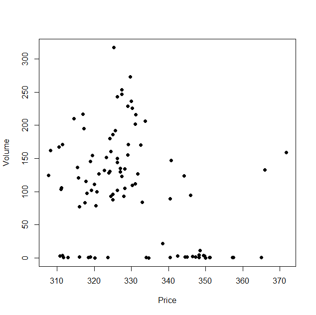
plot(Price, Volume, pch=16)
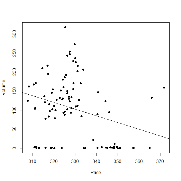
As we see, there seems to be an inverse relationship between the volume traded and the price, as expected. Our goal now is to find a straight line (and its equation), that best fits our observed data, as pictured below. The simplest way of doing so is the so-called “ordinary least squares” regression. As you can see on the graph below, none of our observed data points actually lie on this demand curve, but this line represents the best fit in that it minimizes the total squared distance of each data point from the regression line.

In R, we can estimate the equation of this line as follows:
reg <- lm(Volume~Price, data=data)
summary(reg)


Residuals:
    Min      1Q  Median      3Q     Max
-134.19  -64.72   -3.84   46.73  206.41

Coefficients:
            Estimate Std. Error t value Pr(>|t|)
(Intercept) 683.2323   192.0448   3.558 0.000588 ***
Price        -1.7595     0.5825  -3.021 0.003247 **
---
Signif. codes:  0 ‘***’ 0.001 ‘**’ 0.01 ‘*’ 0.05 ‘.’ 0.1 ‘ ’ 1

Residual standard error: 78.44 on 94 degrees of freedom
Multiple R-squared:  0.08849,   Adjusted R-squared:  0.07879
F-statistic: 9.125 on 1 and 94 DF,  p-value: 0.003247
This regression output tells us that our demand equation was estimated as
Quantity = 683.23 – 1.76*Price
This means that our equation has an intercept of 683.23 and a slope of -1.76. In plain English, if price is equal to 0, then 683230 units will be sold (keeping in mind that our volume variable was measured in thousands, hence we need to multiply our intercept by 1000). If price increases by $1, then quantity demanded decreases by 1760 units.
Besides the demand equation, economists often estimate the price elasticity of demand, which measures the responsiveness of demand to price changes. Formally, elasticity of demand is defined as the percentage change in quantity demanded divided by the percentage change in price. This means, if elasticity of demand is equal to -2, a 1% increase in price will lead to a 2% decrease in quantity demanded. To estimate this elasticity, we will first take the natural logarithm of both our quantity and our price variable. Our estimated equation will then look like this:
ln(Quantity) = b_0+b_1*ln(Price)
Now we need one step of calculus (just bear with me here!) to see how this regression equation gives us the desired elasticity. Taking the total differential of our equation yields
d Quantity/Quantity = b_1*d Price/Price or
b_1 = d Quantity/ d Price * P/Q,
which is exactly the definition of elasticity of demand! Thus, the coefficient b_1 on our log price variable estimates price elasticity of demand. In R, we can do this with the following code:
#Create the logged variables
log_price=log(Price)
log_volume=log(Volume)
#run the log-log regression
reg2 <- lm(log_volume~log_price, data=data)
summary(reg2)

Residuals:
    Min      1Q  Median      3Q     Max
-6.7162 -1.6407  0.9167  1.4937  4.0767

Coefficients:
            Estimate Std. Error t value Pr(>|t|)
(Intercept)  116.523     34.168   3.410 0.000958 ***
log_price    -19.521      5.895  -3.312 0.001317 **
---
Signif. codes:  0 ‘***’ 0.001 ‘**’ 0.01 ‘*’ 0.05 ‘.’ 0.1 ‘ ’ 1

Residual standard error: 2.372 on 94 degrees of freedom
Multiple R-squared:  0.1045,    Adjusted R-squared:  0.09496
F-statistic: 10.97 on 1 and 94 DF,  p-value: 0.001317
We find that our elasticity of demand is equal to -19.5; that is, if price increases by 1%, quantity demanded decreases by 19.5%. Demand for corn futures thus appears to be rather responsive to price changes.
One issue that we have ignored so far is that prices and quantities traded are the result of the interaction of supply and demand in a competitive market. Therefore we cannot be sure that all the data points in our sample lie on the same demand curve, as both the demand and the supply curve may have shifted. Therefore, we may want to use more advanced techniques to account for that – which is a story for another day!
To learn more about demand curves and how to estimate relationships between variables, become a Buff and take courses in microeconomics, econometrics, or quantitative analysis!
Eric Hoffmann
Assistant & Pickens Professor of Economics


