We’ve all heard economists and analysts utter the expression, “It’s all simple supply and demand!” when trying to explain some market phenomenon. Maybe you’ve taken an introductory course in economics. You came to understand how a supply curve and a demand curve cross in order to produce an equilibrium price and quantity. As we know, those equilibrium points change as the supply and demand curves shift.
I’m here to tell you that this entire model is wrong.
Wait, What?
The entire problem centers around the concept of a supply curve. Let’s take a step back in order to examine what’s going on. A supply curve answers this question: Given a market price, what quantity of the good will a firm supply to the market?
At first glance, there doesn’t seem to be anything wrong with asking such a question. Suppose that we went to a local business and asked them how much output they would choose to produce. Assume the possible prices were, say, $2, $5, and $8. Suppose they answer 5 units, 9 units, and 12 units, respectively. You could plot these data points in a graph like the following:
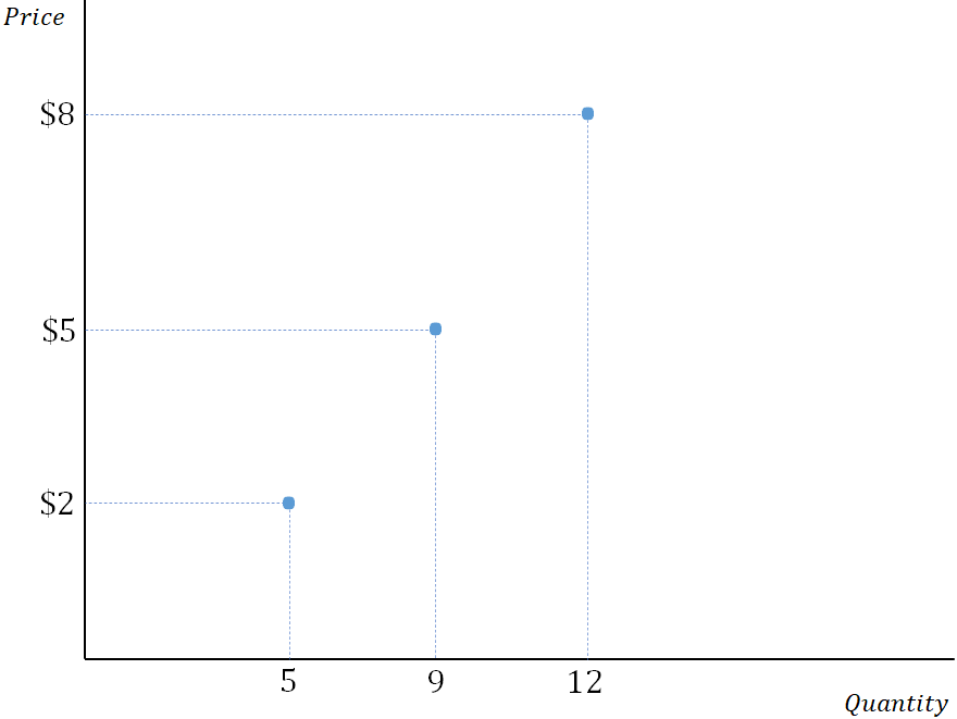
Now, if we were to hypothetically ask them the same question about all possible prices and record their responses, you would get what we call a “supply curve.” This line which lets us know how much will be supplied at any price we could possibly ask about.
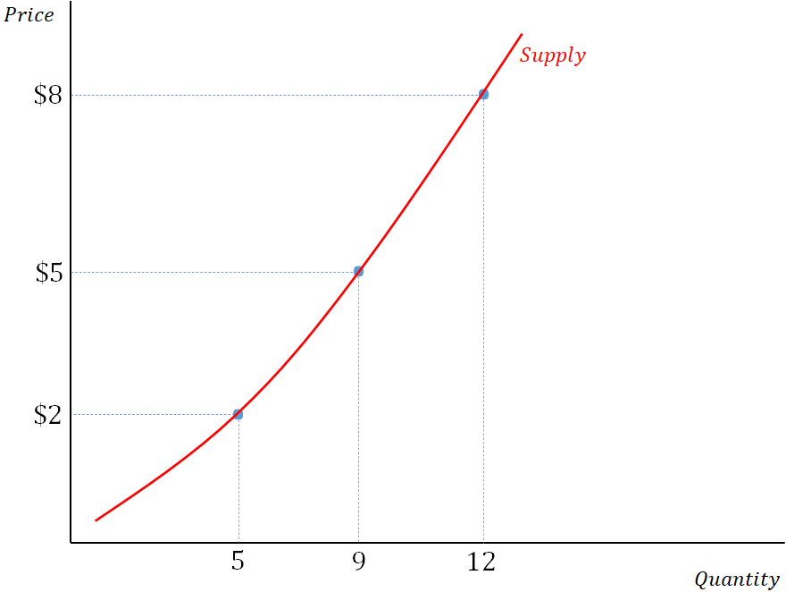
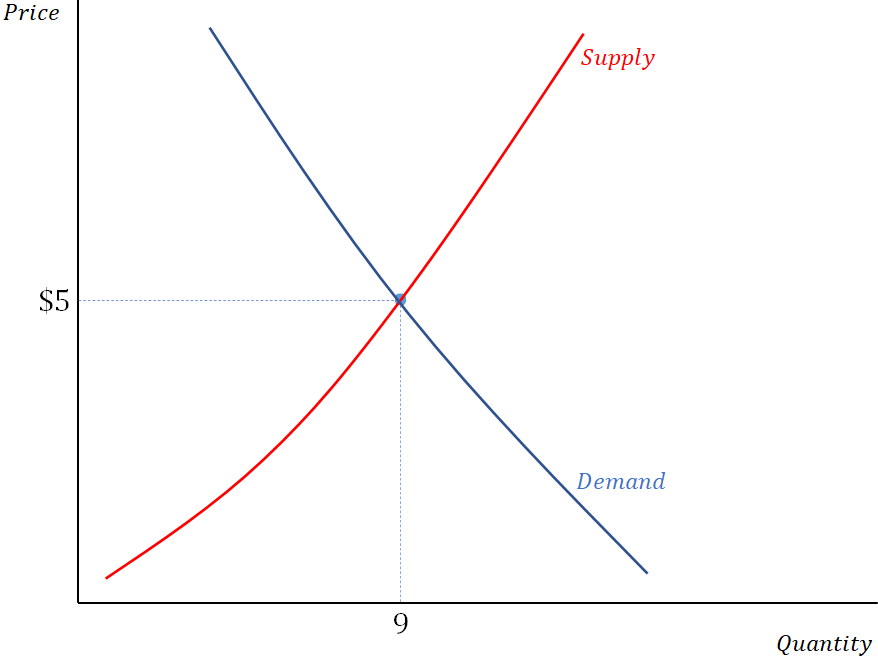
Once we have done that, we can add in our demand curve. This will tell us how much consumers desire to purchase at any given price. We then have our famous supply and demand model. The equilibrium price and quantity ($5 and 9 units for the sake of this example) are determined where the two curves intersect. This looks something like the following:
Is There A Problem With This?
So, where is the problem? Well, in one very special case, which we call the case of perfect competition, there is no problem. In perfect competition, each firm is assumed to be very small. Furthermore, no matter how much it decides to produce, the price being offered by consumers is unaffected.
For example, suppose I am a small corn farmer in Kansas. Assume there are currently 100 million units of corn being produced on the world market, for which consumers are willing to offer $2 a unit. Then, assume that I decide that it is optimal for me to produce 1,000 units of corn at this $2 price. My extra thousand units is unlikely to affect market demand in such a way as to result in a price change. This lack of “market power” allows us to isolate this particular market price and accurately record what I would produce.
It’s Complicated
Things get more complicated beyond the case of perfect competition, however, and it turns out that the above exercise becomes impossible to carry out. To see why, consider two large-scale oil producers (firms 1 and 2, respectively). Their output decisions make a large enough impact on the world market so as to affect the market price.
To make things concrete, suppose that the price which consumers are willing to pay for a certain amount of output. This is nothing more than the demand curve, and is given by the equation
P = 17-(Q1+ Q2)
In this equation, P is price, and Q1 and Q2 are how much output firms 1 and 2 produce, respectively.
Let’s Juggle The Numbers
Now let’s ask each firm how much they would like to produce if the market price were $5. Suppose that firm 1 answers with 9 units of output, as in our previous example. Suppose then that firm 2 declares that they would like to like to produce 8 units of output. But upon learning firm 2’s output decision, which we now assume is able to affect market price, firm 1’s profit maximizing production decision may change. Hence, firm 1 may decide to change their output decision from 9 units to, say, 4 units.
But this alters the market price once again, and along with it firm 2’s profit maximizing production decision. They may thus want to change their production level from 8 units to something else. At the end of the day, this back and forth competition will eventually result in some equilibrium production level for both firms. For example, it may be Q1 =10 and Q2 =5, which we call a “Nash equilibrium.” But when we plug these output levels back into the demand function, the resulting market price is
P = 17-(Q1+ Q2) = 17 – (10+5) = $2
Thus, the market price is no longer $5, but rather $2! This leads to an immediate inconsistency, as these output levels no longer answers the original question of what we would expect to be produced at the market price of $5.
Help! I’m Confused!
What is going on here? Very simply, when firms have market power, or the ability to affect the price with their output decisions, any answer to the question “How much would you produce if the price is X?” can result in a back and forth jostling to a Nash equilibrium. This results in a market price other than X.
Formally, we say that prices are endogenously determined, or determined as a result of the firms’ profit maximizing decisions, not prior to. And if you can’t ask this “prior to” question, you can’t get a supply curve, and hence you can’t do traditional supply and demand analysis.
Whatever Shall We Do?
Thankfully, all is not lost. In fact, I will argue that the very supply and demand model which we’ve just shown to be technically incorrect is a useful heuristic for all of the things we care about. To begin, if we are going to throw out the supply and demand model, we need an alternative way to calculate what the market equilibrium and price will be. If you take my ECON 4301-Industrial Organization course, you will learn all about how we do this. To make a long story short, suppose we have a market demand curve given by
P = K – Q
In this equation K is some demand parameter, and Q = Q1+ Q2 +…+ QN is the total market output with N firms. In our above example, we set K=17, and had N=2 firms. But we can abstract away from this and let these numbers be anything we wish. Lastly, suppose firms have a marginal cost of production which we denote by the letter c (which we assume is less than K to make life easy). After a little bit of calculus and algebra to solve for the Nash equilibrium, we can determine that the market price and quantity will be given by the following:

These are not the sorts of equations one usually sees in Econ 101. But if you take a closer look, you will notice they entirely vindicate our old, familiar, and technically incorrect supply and demand model. Let’s see why:
Change 1: Increase in Demand
According to our supply and demand story from Econ 101, an increase in demand should result in an increase in the equilibrium output and price. This is usually represented graphically as:
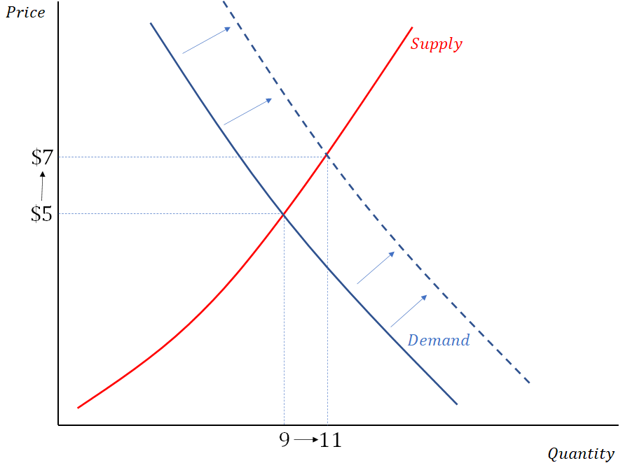
But given our previous discussion, are we to trust this intuition? Yes! It turns out that both P* and Q* from equations 1 and 2 are increasing as the demand parameter K increases. Therefore, the supply and demand model gives the same qualitative equilibrium prediction as do our equilibrium equations. This is true even though the former is technically incorrect.
Change 2: Increase in Costs
Now suppose that the costs of production for firms increase. In our supply and demand story, this will result in a decrease, or backwards shift, of the supply curve. This can be represented graphically as
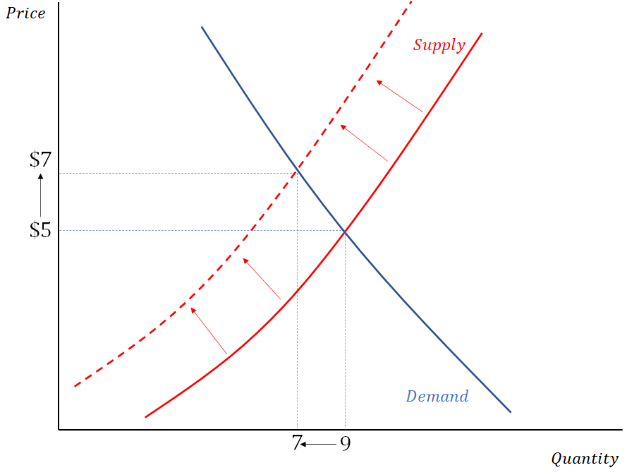
Here, we see that our traditional supply and demand model predicts a higher equilibrium price. It similarly predicts a lower equilibrium quantity after the increase in production costs. Once again, a close examination of equations 1 and 2 reveal that an increase in c will result in an increase in P* and a decrease in Q*! This is almost too good to be true. Let’s do one more.
Change 3: Increase in the Number of Firms
Lastly, let’s consider what happens when the number of firms in the market increases. In our traditional supply and demand graph, this would be represented by an increase, or outward shift, of the supply curve, which we can represent graphically as:
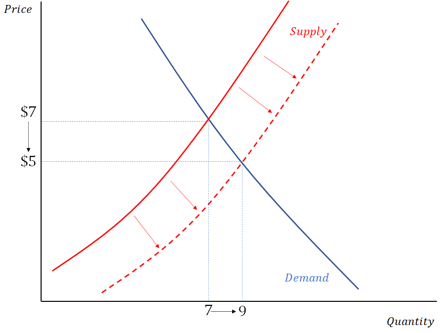
This suggests that as the number of firms increases, we should expect to see a lower market price and more market output in equilibrium. Well, what do you know? As N increases, the term N/(N+1) gets larger, and a close look will reveal that this will result in a decrease in P* and an in Q*! Once again, the supply and demand model produce the same qualitative predictions as what we know to be the correct equilibrium outcome.
In Conclusion…
At the end of the day, what are we to make of all of this? We began with the troubling fact that unless we are in the case of a perfectly competitive market, we cannot make sense of the concept of a supply curve. This renders our traditional supply and demand analysis technically inadequate. However, despite this, it remains a tremendously useful “rule of thumb.” It agrees with all of the qualitative predictions we obtain from the more accurate calculations. In this way, we are perfectly fine explaining economic phenomenon as if a supply curve actually exists.
And this is nice to know, because at the end of the day, it’s all simple supply and demand.
Dr. Eric Hoffmann
Associate and Pickens Professor of Economics


